Seismic Use Cases
Seismic Response of Concrete Walls
Modeling Reinforced Concrete Walls using Shell Elements in OpenSees and Using Jupyter to Post Process Results
Josh Stokley - University of Washington
Laura Lowes - University of Washington
Key Words: OpenSees, Jupyter, HPC
The purpose of this use case is to be able to model, simulate, and post process multiple reinforced concrete walls at once. This use case uses jupyter notebooks to model these walls with shell elements and uses OpenSeesMP on DesignSafe to simulate the models. The documentation of this use case will use a single wall, RW1, as an example to understand the workflow and objectives of this use case.
Resources
Jupyter Notebooks
The following Jupyter notebooks are available to facilitate the analysis of each case. They are described in details in this section. You can access and run them directly on DesignSafe by clicking on the "Open in DesignSafe" button.
| Scope | Notebook |
|---|---|
| Matlab to Python | Matlab_to_Python.ipynb |
| Tcl-Script Creator | TCL_Script_Creator.ipynb |
| Load-Displacement History | DisplacementLoadHistory.ipynb |
| Cross-Sectional Analysis | CrossSectionSteelConcreteProfile.ipynb |
| Movies | Movies.ipynb |
| Crack Angle Viz | CrackedModel.ipynb |
DesignSafe Resources
The following DesignSafe resources were used in developing this use case.
Background
Citation and Licensing
-
Please cite Shegay et al. (2021) to acknowledge the use of any data from this use case.
-
Please cite Lu XZ et al. (2015) to acknowledge the use of the modeling strategy from this use case.
-
Please cite Rathje et al. (2017) to acknowledge the use of DesignSafe resources.
-
This software is distributed under the GNU General Public License .
Description
Data
The walls that are modeled are defined in a database provided by Alex Shegay. The database is a MATLAB variable of type 'structure'. The tree-like structure of the variable consists of several levels. Each level consists of several variables, each being a 1x142 dimension array. Each entry within the array corresponds to a separate wall specimen. The order of these entries is consistent throughout the database and reflects the order of walls as appearing in the 'UniqueID' array.
Modeling
The modeling techniques are inspired by the work of Lu XZ. The modeling of these walls make use of the MITC4 shell element. This element smears concrete and steel in multiple layers through the thickness of the element. Figure 1 demonstrates this. Within the shell element, only the transverse steel is smeared with the concrete. The shell elements are modeled to be square or close to square for best accuracy, an assumption that follows this is that cover concrete on the ends of the wall are not taken into account as it would produce skinny elements that would cause the wall to fail prematurely. The vertical steel bars are modeled as trusses up the wall to better simulate the stress of those bars. The opensees material models that are used are:
-
PlaneStressUserMaterial- Utilizes damage mechanisms and smeared crack model to define a multi-dimensional concrete model
- Variables include: compressive strength, tensile strength, crushing strength, strain at maximum and crushing strengths, ultimate tensile strain, and shear retention factor
- Model can be found in Lu XZs citation
-
Steel02- Uniaxial steel material model with isotropic strain hardening
- Variables include: yield strength, initial elastic tangent, and strain hardening ratio
- Model can be found here: Steel02 OpenSees

Figure 1: Smeared shell element representation
Example
RW1 is modeled from the database to produce a tcl file that represents the geometry, material, and simulation history of the wall. The wall is 150 inches high, 46.37 inches long, and 4 inches thick. It consists of 1292 amount of nodes, 1200 amount of shell elements, and 900 amount of steel truss elements. MITC4 shell elements are used to smear the concrete and transverse steel into the thickness while the vertical reinforce bars are modeled as truss elements. RW1 had a compression buckling failure mode in the lab. More information on RW1 and its experimental results can be found here: Wallace et al. (2004)
The use case workflow involves the following steps:
- Using Jupyter notebook modeling script to create input file for OpenSees
- Running input file through HPC on DesignSafe
- Using Jupyter notebook post processing scripts to evaluate model
Create Input File using Modeling Script
The modeling script is broken up into 2 notebooks, the first notebook imports the variables to build the wall into an array. The second notebook builds out the tcl file that will be ran through openseees. The sections defined below are from the second notebook.
The matlab to python script can be found here: Matlab_to_Python.ipynb
The jupyter notebook that creates the OpenSees input file can be found here: TCL_Script_Creator.ipynb
Reinforced Concrete Wall Database
Each wall in the database has a number corresponding to its unique ID. This number will be the single input to the modeling script to create the script. The use case will loop through multiple numbers to create multiple files at once and run them through opensees. Variables are separated in the database by sections. For example, under the section 'Geometry', one can find the heights of the walls, the thickness of walls, the aspect ratios, and so on. By parsing through these sections, the necessary information can found and imported into the modeling script to build out the wall.
RW1 is wall 33 in the database (with the first wall index starting at 0) and using that index number, the modeling script can grab everything that defines RW1.
Modeling Script
The sections of the modeling script are:
Section 1: Initialization of the model
- The degrees of freedom and the variables that carry uncertainty are defined.
Section 2: Defines nodal locations and elements
- Nodes are placed at the locations of the vertical bars along the length of the wall.
- If the ratio of the length of the wall to the number of elements is too coarse of a mesh, additional nodes are placed in between the bars.
- The height of each element is equal to the length of the nodes in the boundary to create square elements up the wall.
Section 3: Defines material models and their variables
- The crushing energy and fracture energy are calculated and wrote to the .tcl file. The equations for these values come from (Nasser et al. (2019) ) Below is the code:
self.gtcc = abs((0.174*(.5)**2-0.0727*.5+0.149)*((self.Walldata[40]*1000*conMult)/1450)**0.7) #tensile energy of confined
self.gtuc = abs((0.174*(.5)**2-0.0727*.5+0.149)*((self.Walldata[40]*1000)/1450)**0.7) # tensile energy of unconfined
self.gfuc = 2*self.Walldata[40]*6.89476*5.71015 #crushing energy of unconfined
self.gfcc = 2.2*self.gfuc #crushing energy of confined- The crushing strain (epscu) and fracture strain (epstu) can then be calculated from the energy values.
- The material models are then defined.
- The concrete material opensees model: nDmaterial PlaneStressUserMaterial $matTag 40 7 $fc $ft $fcu $epsc0 $epscu $epstu $stc.
- 'fc' is the compressive strength, 'ft' is the tensile strength, 'fcu' is the crushing strength, and 'epsc0' is the strain at the compressive strength.
- The steel material opensees model: uniaxialMaterial Steel02 $matTag $Fy $E $b $R0 $cR1 $cR2.
- 'Fy' is the yield strength, 'E' is the youngs modulus, 'b' is the strain hardening ratio, and 'R0', 'cR1', and 'cR2' are parameters to control transitions from elastic to plastic branches.
- minMax wrappers are applied to the steel so that if the steel strain compresses more than the crushing strain of the concrete or exceeds the ultimate strain of the steel multiplied by the steel rupture ratio, the stress will go to 0.
Section 4: Defines the continuum shell model
- The shell element is split up into multiple layers of the cover concrete, transverse steel, and core concrete.
- The cover concrete thickness is defined in the database, the transverse steel thickness is calculated as:
- total layers of transverse steel multiplied by the area of the steel divided by the height of the wall.
- The total thickness of the wall is defined in the database so after the cover concrete and steel thicknesses are subtracted, the core concrete takes up the rest.
Section 5: Defines the elements
- The shell element opensees model is: element ShellMITC4 $eleTag $iNode $jNode $kNode $lNode $secTag
- 'eleTag' is the element number, the next four variables are the nodes associated to the element in ccw, and 'secTag' is the section number that defines the thickness of the element.
- There are usually two sections that are defined, the boundary and the web. Based on how many nodes are in the boundary, the script will print out the elements for the left side of the boundary, then for the entire web region, and lastly for the right side of the boundary. This process is repeated until the elements reach the last row of nodes.
- For the vertical steel bars, the truss element opensees model is used: element truss $eleTag $iNode $jNode $A $matTag.
- The node variables are defined as going up the wall so if a wall has 10 nodes across the base, the first truss element would connect node 1 to node 11.
- 'A' is the area of the bar and 'matTag' is the material number applied to the truss element.
- The script prints out truss elements one row at a time so starting with the left furthest bar connecting to each node until the height of the wall is reached and then next row is started the bar to the right.
Section 6: Defines constraints
- The bottom row of nodes are fixed in all degrees of freedom.
Section 7: Defines recorders
- The first two recorders capture the force reactions in the x-direction of the bottom row of nodes and the displacements in the x-direction of the top row of nodes. These recorders will be used to develop load-displacement graphs.
- The next eight recorders capture stress and strain of the four gauss points in the middle concrete fiber of all the elements and store them in an xml file. These recorders will be used to develop stress and strain profile movies, give insight to how the wall is failing, and how the cross section is reacting.
- The last two recorders capture the stress and strain of all the truss elements. These will be used to determine when the steel fails and when the yield strength is reached.
- Recorders are defined as below where 'firstRow' and 'last' are the nodes along the bottom and top of the wall 'maxEle' is the total amount of shell elements and 'trussele' is the total elements of shell elements and truss elements in the wall.
self.f.write('recorder Node -file baseReactxcyc.txt  -node {}  -dof 1 reaction\n'.format(' '.join(firstRow)) )
self.f.write('recorder Node -file topDispxcyc.txt    -node {}  -dof 1 disp \n'.format(' '.join(last)))
self.f.write('recorder Element -xml "elementsmat1fib5sig.xml"  -eleRange 1 ' + str(self.maxEle) + ' material 1    fiber 5    stresses\n')
self.f.write('recorder Element -xml "elementsmat2fib5sig.xml"  -eleRange 1 ' + str(self.maxEle) + ' material 2    fiber 5    stresses\n')
self.f.write('#recorder Element -xml "elementsmat3fib5sig.xml"  -eleRange 1 ' + str(self.maxEle) + ' material 3    fiber 5    stresses\n')
self.f.write('#recorder Element -xml "elementsmat4fib5sig.xml"  -eleRange 1 ' + str(self.maxEle) + ' material 4    fiber 5    stresses\n')
self.f.write('recorder Element -xml "elementsmat1fib5eps.xml"  -eleRange 1 ' + str(self.maxEle) + ' material 1    fiber 5    strains\n')
self.f.write('recorder Element -xml "elementsmat2fib5eps.xml"  -eleRange 1 ' + str(self.maxEle) + '  material 2    fiber 5    strains\n')
self.f.write('#recorder Element -xml "elementsmat3fib5eps.xml"  -eleRange 1 ' + str(self.maxEle) + '  material 3    fiber 5    strains\n')
self.f.write('#recorder Element -xml "elementsmat4fib5eps.xml"  -eleRange 1 ' + str(self.maxEle) + ' material 4    fiber 5    strains\n')
self.f.write('recorder Element -xml "trusssig.xml"  -eleRange ' + str(self.maxEle+1) + ' ' + str(self.trussele)+ ' material stress\n')
self.f.write('recorder Element -xml "trussseps.xml" -eleRange ' + str(self.maxEle+1) + ' ' + str(self.trussele)+ ' material strain\n')
Section 8: Defines and applies the gravity load of the wall
- The axial load of the wall is defined in the database and distributed equally amongst the top nodes and a static analysis is conducted to apply a gravity load to the wall.
Section 9: Defines the cyclic analysis of the wall
- The experimental displacement recording of the wall is defined in the database and the peak displacement of each cycle is extracted.
- If the effective height of the wall is larger than the measured height, a moment is calculated from that difference and uniformly applied in the direction of the analysis to each of the top nodes.
- The displacement peaks are then defined in a list and ran through an opensees algorithm.
- This algorithm takes each peak and displaces the top nodes of the wall by 0.01 inches until that peak is reached, it then displaces by 0.01 inches back to zero where it then takes on the next peak. This process continues until failure of the wall or until the last peak is reached.
The last section of this notebook creates a reference file that holds variables needed for postprocessing. In order, those variables are: * Total nodes along the width of the wall * Total nodes along the width of the wall that are connected to a truss element * Total nodes in the file * Total elements in the file * Displacement peaks in the positive direction * Fracture strength of the concrete * total layers of elements in the file * Unique ID of the wall * filepath to the folder of the wall * filepath to the tcl file
Running Opensees through HPC
(Script needs to be established on design safe. I have a working notebook, just need to connect it with modeling script)
Post Processing
After the script is finished running through OpenSees, there are multiple post-processing scripts that can be used to analyze the simulation and compare it to the experimental numbers.
Load-Displacement Graph
The Load-Displacement script compares the experimental cyclic load history to the simulated cyclic load output. The x axis is defined as drift % which is calculated as displacement (inches) divided by the height of the wall. The y axis is defined as shear ratio and calculated as force (kips) divided by cross sectional area and the square root of the concrete compressive strength. This Script can be found here: DisplacementLoadHistory.ipynb

Cross Sectional Analysis of Concrete and Steel
The cross sectional script shows stress and strain output across the cross section of the first level for the concrete and steel at various points corresponding with the positive displacement peaks. This script can be found here: CrossSectionSteelConcreteProfile.ipynb

Stress and Strain Profile Movies
The Stress/Strain profile movie script utilizes plotly to create an interactive animation of stresses and strains on the wall throughout the load history. The stress animations are vertical stress, shear stress, and maximum and minimum principal stress. The strain animations are vertical strain, shear strain, and maximum and minimum principal strain. This script can be found here: Movies.ipynb

Crack Angle of Quadrature Points
The crack angle script will show at what angle each quadrature point cracks. When the concrete reaches its fracture strength in the direction of the maximum principal stress, it is assumed that it cracked and the orientation at that point is then calculated shown on the graph. The blue lines indicates the crack angle was below the local x axis of the element and the red line means the crack angle was above the local x axis of the element. This script can be found here: CrackedModel.ipynb

Soil Structure Interaction
Integration of OpenSees-STKO-Jupyter to Simulate Seismic Response of Soil-Structure-Interaction
Yu-Wei Hwang - University of Texas at Austin
Ellen Rathje - University of Texas at Austin
Key Words: OpenSees, STKO, Jupyter, HPC
This use case example shows how to run an OpenSeesMP analysis on the high-performance computing (HPC) resources at DesignSafe (DS) using the STKO graphical user interface and a Jupyter notebook. The example also post-processes the output results using python scripts, which allows the entire analysis workflow to be executed within DesignSafe without any download of output.
Resources
Jupyter Notebooks
The following Jupyter notebooks are available to facilitate the analysis of each case. They are described in details in this section. You can access and run them directly on DesignSafe by clicking on the "Open in DesignSafe" button.
| Scope | Notebook |
|---|---|
| Submit job to STKO-compatible OpenSees | SSI_MainDriver.ipynb |
| Post-Processing in Jupyter | Example post-processing scripts.ipynb |
DesignSafe Resources
The following DesignSafe resources were used in developing this use case.
Background
Citation and Licensing
-
Please cite Hwang et al. (2021) to acknowledge the use of any resources from this use case.
-
Please cite Rathje et al. (2017) to acknowledge the use of DesignSafe resources.
-
This software is distributed under the GNU General Public License .
Description
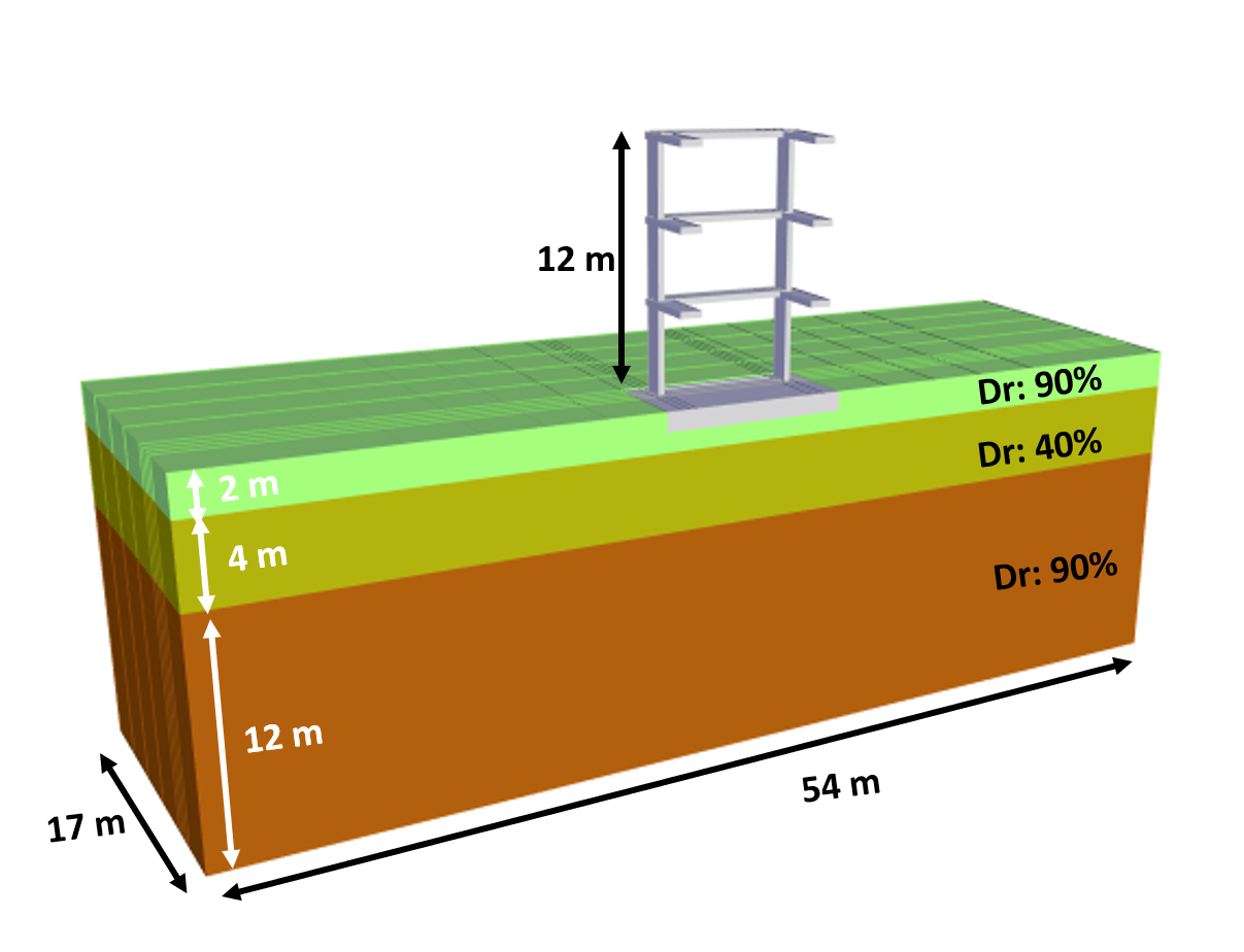
A hypothetical three dimensional soil–foundation–structure system on liquefiable soil layer is analyzed using OpenSees MP. The soil profile first included a 12-m thick dense sand layer with Dr of 90%, followed by a 4-m thick loose sand layer with Dr of 40%, and overlaid by a 2-m thick dense sand layer. The ground water table was at ground surface. An earthquake excitation was applied at the bottom of the soil domain under rigid bedrock conditons. A three-story, elastic structure was considered on a 1-m-thick mat foundation. The foundation footprint size (i.e., width and length) was 9.6m x 9.6m with bearing pressure of 65 kPa. Additional information can be found in Hwang et al. (2021)
The use case workflow involves the following steps:
-
Creating the OpenSees input files using STKO.
-
Submitting the OpenSees job to the Stampede2 HPC resources at DesignSafe/TACC.
-
Post-processing the results using STKO and python.
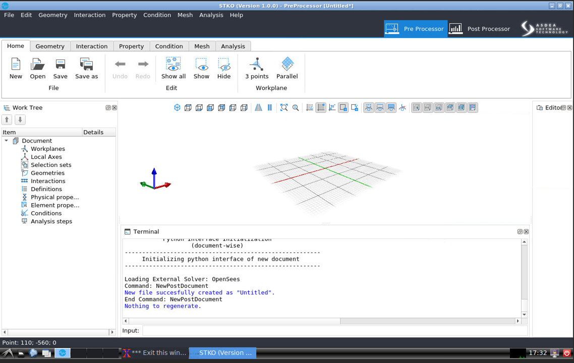
Create OpenSees Model using STKO
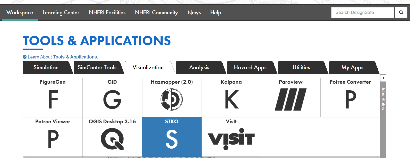
- The user can create the input OpenSees-STKO model (both the 'main.tcl' and 'analysis_steps.tcl' files, as well as the '*.cdata' files) using STKO , which is available from the Visualization tab of the Tools & Applications section of the DesignSafe Workspace.
- Save all the files (tcl script and mpco.cdata files) in a folder under the user's My Data directory within the Data Depot.
- Alternatively, the input OpenSees-STKO model can be created on the user's local computer and all the files uploaded to a My Data folder.
Setup and submit OpenSees job via Jupyter notebook
A Jupyter notebook, SSI_MainDriver.ipynb , is provided that submits a job to the STKO compatible version of OpenSeesMP.
This Jupyter notebook utilizes the input file 'main.tcl', as well as 'analysis_steps.tcl' and the associated '*.cdata' files created by STKO. All of these files must be located in the same folder within the My Data directory of the DesignSafe Data Depot.
Setup job description
This script demonstrates how to use the agavepy SDK that uses the TAPIS API to setup the job description for the OpenSeesMP (V 3.0) App that is integrated with STKO. More details of using TAPIS API for enabling workflows in Jupyter notebook can be found in the DesignSafe webinar: Leveraging DesignSafe with TAPIS
- The user should edit the "job info" parameters as needed.
- The "control_jobname" should be modified to be meaningful for your analysis.
- The "control_processorsnumber" should be equal to the "number of partitions" in the STKO model.
from agavepy.agave import Agave
ag = Agave.restore()
import os

### Running OPENSEESMP (V 3.0)-STKO ver. 3.0.0.6709
app_name = 'OpenSeesMP'
app_id = 'opensees-mp-stko-3.0.0.6709u1'
storage_id = 'designsafe.storage.default'

##### One can revise the following job info ####
control_batchQueue = 'normal'
control_jobname = 'SSI_NM_Northridge_0913'
control_nodenumber = '1'
control_processorsnumber = '36'
control_memorypernode = '1'
control_maxRunTime = '24:00:00'
Submit and Run job on DesignSafe
The script below submits the job to the HPC system.
job = ag.jobs.submit(body=job_description)
print("Job launched")import time
status = ag.jobs.getStatus(jobId=job["id"])["status"]
while status != "FINISHED":
status = ag.jobs.getStatus(jobId=job["id"])["status"]
print(f"Status: {status}")
time.sleep(3600)Identify Job ID and Archived Location
After completing the analysis, the results are saved to an archive directory. This script fetches the jobID and identifies the path of the archived location on DS.
jobinfo = ag.jobs.get(jobId=job.id)
jobinfo.archivePath
user = jobinfo.archivePath.split('/', 1)[0]jobinfo.archivePath
'$username/archive/jobs/job-3511e755-cb3f-4e3e-92b9-615cc40d39e6-007'Post-processing on DesignSafe
The output from an OpenSeesMP-STKO analysis are provided in a number of '*.mpco' files, and these files can be visualized and data values extracted using STKO. Additionally, the user can manually add recorders to the 'analysis_steps.tcl' file created by STKO and the output from these recorders will be saved in *.txt files. These *.txt can be imported into Jupyter for post-processing, visualization, and plotting.
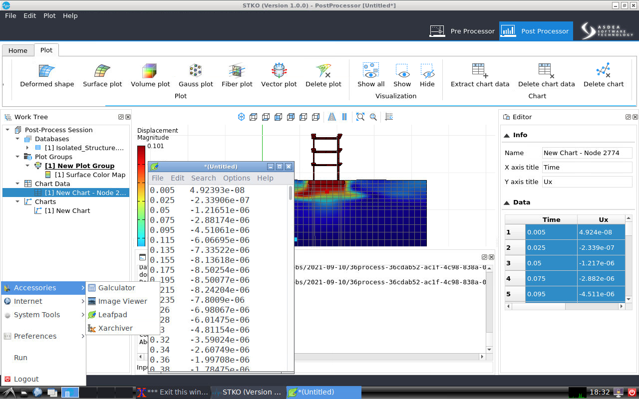
Visualize and extract data from STKO
After the job is finished, the user can use STKO to visualize the results in the '*.mpco' files that are located in the archive directory. If the user would like to extract data from the GUI of STKO, they can copy and paste the data using the "Leafpad" text editor within the DS virtual machine that serves STKO. The user can then save the text file to a folder within the user's My Data directory.
Example post-processing scripts using Jupyter
A separate Jupyter notebook is provided (Example post-processing scripts.ipynb ) that post-processes data from OpenSees recorders and save in *.txt files. The Jupyter notebook is set up to open the *.txt files after thay have been copied from the archive directory to the same My Data in which the notebook resides.
For this example, recorders are created to generate output presented in terms of:
-
Acceleration response spectra at the mid of loose sand layer, foundation, and roof.
-
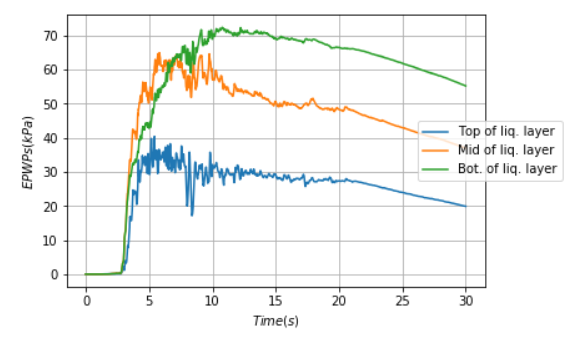
Evolution of excess pore water pressure at the bottom, mid, and top of the loose sand layer.
-
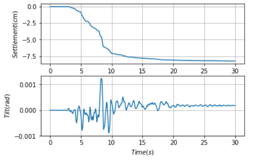
Time history of foundation settlement and tilt.
Creating recorders
To manually add the recorders, the user needs to first identify the id of the nodes via STKO (see StruList and SoilList below) and their corresponding partition id (i.e., Process_id). These recorders should be added into the "analysis_steps.tcl" before running the model. Note that the "analysis_steps.tcl" is automatically generated by STKO.
if {$process_id == 20} {
set StruList {471 478 481}
eval "recorder Node -file $filename.txt -time -node $StruList -dof 1 3 -dT $timestep disp"
eval "recorder Node -file $filename.txt -time -node $StruList -dof 1 -dT $timestep accel"

set SoilList {2781}
eval "recorder Node -file $filename.txt -time -node $SoilList -dof 1 3 -dT $timestep disp"
eval "recorder Node -file $filename.txt -time -node $SoilList -dof 1 -dT $timestep accel"
eval "recorder Node -file $filename.txt -time -node $SoilList -dof 4 -dT $timestep vel"
}
Example Post-processing Results
This section shows the results from the post-processing scripts performed via the Jupyter notebook. The notebook is broken into segments with explanations of each section of code. Users should edit the code to fit their own needs.
Response spectra for motions at various locations within the model
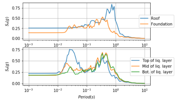
Time history of excess pore pressure at different locations in the soil
Time history of foundation settlement and tilt
Experimental Shake Table Testing
Integrated Workflow of Experiments using Jupyter Notebooks: From Experimental Design to Publication
Enrique Simbort - University of California, San Diego
Gilberto Mosqueda - University of California, San Diego
Key Words: Jupyter, Interactive Data Analysis, UCSD NHERI Facility
Jupyter Notebooks can provide fully integrated workflows of experiments from documentation of experimental design through analysis and publishing of data using the DesignSafe cyberinfrastructure. A series of Notebooks are being developed to demonstrate their use in the experimental workflow including notebooks showing how to view and analyzed past published data and data from testing of a reconfigurable, modular test bed building planned to be tested on the NHERI@UC San Diego Experimental Facility. The Python-based code is implemented in a modular fashion so that components can be used as desired in other experiments and are transferable to other experimental facilities. In the examples provided, the Notebook can be used to evaluate shake table performance as well as dynamic properties of the structure. A key functionality is to increase the integration and collaboration between researchers at local or remote sites to view and analyze the experimental data during and after testing including after the data is published. As Notebooks are developed to view experimental data by the research team, they can also be published with the data allowing other researchers to quickly view the data for promoting data reuse. Examples are providing for viewing data from past shake table experiments including NEES and more current NHERI data repositories.
Resources
Jupyter Notebooks
The following Jupyter notebooks are available to facilitate the analysis of each case. They are described in details in this section. You can access and run them directly on DesignSafe by clicking on the "Open in DesignSafe" button.
| Scope | Notebook |
|---|---|
| Shake-Table Performance | Case 1. Shake table performance.ipynb |
| Structural Response and System Identification | Case 2: Structural Response and System Identification.ipynb |
| Experimental Workflow | Case 3: Experimental Workflow.ipynb |
DesignSafe Resources
The following DesignSafe resources were used in developing this use case.
Background
Citation and Licensing
- Please cite Mosqueda et al. (2017) to acknowledge the use of resources from this use case with additional data sources referenced below.
- Please cite Rathje et al. (2017) to acknowledge the use of DesignSafe resources.
- This software is distributed under the GNU General Public License .
Description
As the cyberinfrastructure for The Natural Hazard Engineering Research Infrastructure (NHERI), DesignSafe, see Rathje et al. (2020) , provides a collaborative workspace for cloud-based data analysis, data sharing, curation and publication of models and data. Within this workspace, Jupyter Notebooks can be applied to perform data analysis in an interactive environment with access to published data. A rich set of data from natural hazard experiments and field studies is available from NHERI projects and its predecessor the Network for Earthquake Engineering Simulation (NEES). Since one of the major goals of DesignSafe is to provide a collaborative workspace by means of data sharing and access for data reuses, the main objective of this document is to demonstrate the use of Jupyter Notebook for viewing and analyzing published data using cloud-based tools.
This use case includes a series of Jupyter Notebooks aimed to serve as a learning tool for viewing and analyzing data from shake table experiments including:
-
The first module examines the performance of Hybrid Simulation Experiments conducted on the 1D Large High Performance Outdoor Shake table at UC San Diego with the data published in DesignSafe by Vega et al. (2018) . This module focuses on the response of the shake table including tools to compare different signals. Data extraction and processing of measured sensor data includes comparison of time history signals, comparison of signals in the frequency domain using FFT and comparison of response spectra that show for example target and measured table response.
-
The second module examines the use of Jupyter Notebooks including Python libraries for structural response and system identification. In this case data from a past NEES experiment conducted by Mosqueda et al. (2017) of three-story moment frame structure is examined. The data published in DataDepot under as a NEES project. Using selected sensors at each story of the structure and white noise excitation, the frequencies and mode shapes of the structure are identified. The processing tools rely on existing libraries in Python demonstrating the wealth of access to subroutine that can be applied for analysis.
-
The third module is a Jupyter notebook for viewing and analyzing data from tests on a 3-story steel Modular Testbed Building (MTB2) conducted on the recently upgrades 6DOF shake table at the UC San Diego NHEIR Experimental Facilty as reported by Van Den Einde et al (2020) . These tests will examine the shake table performance and structural response for the 3D structure. These tests are currently in progress with the notebook under development concurrently.
Jupyter Notebooks for Experimental Data
Jupyter Notebooks work as an interactive development environment to code and view data in a report format. Within the notebook, the combination of cells enables formatted text and interactive plotting for viewing and analyzing data. Users can select data files and data channels for viewing and processing with the ability to view and print complete reports. Jupyter Notebooks are accessible in DesignSafe through the workspace analysis tools and can access private or public data in Data Depot. Sample modules are presented here that have been developed using published data in Data Depot including those by Vega et al. (2018) and Masroor et al. (2010) . These modules will be configured and applied within the workflow of the MTB2 during shakedown testing.
Case 1. Shake table performance
A set of modules have been developed to evaluate the performance of the shake table using data from past experiments conducted to demonstrate the hybrid testing capabilities of LHPOST, see Vega et al (2020) . For these hybrid tests, separate Jupyter Notebooks have been developed to consider the various sources of generated data including i) Shake Table Controller, ii) the primary Data Acquisition System (DAQ), and iii) additional computational sources for hybrid testing. In a typical shake table test, the first two sources of data would be included plus any other user specified data acquisition system.
Data collected by the shake table controller is expected to be standard across most tests and useful to verify the performance of the shake table in reproducing the ground motions. Here, data from the shake table controller is used to compare reference command and measured feedback data to evaluate the fidelity of the shake table in reproducing the desired ground motions, see Vega et al. (2018) for an example. The Jupyter notebook functionality includes interactive plotters for viewing either a single channel or multiple channels to compare the reference input and feedback, for example, by viewing the time history, Fourier Transform or Response Spectra (Fig 1). The shake table controller sampling rate was set to a frequency of 2048 [Hz] for this test. Initial implementation of the code required about 3.5 minutes to run. To improve the run-time, various options were explored including down sampling and use of tools such as those being developed by Brandenberg, S., J., & Yang, Y. (2021) to calculate the spectral acceleration. By using these tools, the run time was reduced to approximately 10 s. The module was implemented for the previous 1-D capability of LHPOST but can be easily extended for its newly upgraded 6DOF capabilities.

Figure 1. Evaluation of shake table performance through comparison of command reference and feedback including a) Fourier Transform and b) response spectra .
Case 2. Module for Structural Response and System Identification
The primary goal of the structural response module is to quickly and accurately analyze experimental data. For development and testing of available algorithms, experimental data from a previous dynamic experiment involving a ¼ scale three-story steel moment frame structure were used. For detailed information see Mosqueda et al. (2017) , with the data available in Masroor et al. (2010) . A cross spectral density function (CSD) is applied to compare the white noise acceleration input at the platen to the acceleration at each floor. To improve code clarity and compatibility for future investigators, the CSD function from the SciPy signal package, developed by Virtanen et al (2020) , is implemented, which is well documented. The CSD for each floor is plotted using the matplotlib library. The resulting CSD plots are shown up to 20 Hz in Fig. 2 and identify the natural frequencies of the structure. Modal displacements can also be calculated directly from the CSD function outputs. This is accomplished by using the frequency-power relation between acceleration spectral density functions and displacement spectral density functions. The modal displacements for each story occur at frequencies where the CSD has a local maximum. To obtain these values for the test data of the three-story structure, the frequencies of the first three local maxima were recorded. For future use of this code, the desired number of mode shapes can be scaled by adding or removing local maxima terms at the start of the mode shapes code section. Using the CSD function does not take into account the sign of the modal displacement, however, since these functions are strictly positive over their domain. To account for this, the output of the CSD function at the local maxima frequencies is reexamined without considering the absolute values of its components to identify if the parameters yield a negative number at the corresponding frequency. The rough shape of the modal displacements is plotted as shown in Fig. 3. Future work for this notebook includes generating a smoothing function for the mode shapes and comparison of data from different tests to identify changes in dynamic properties through the testing series that could be indicative of damage.
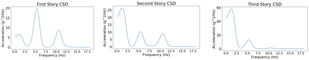
Figure 2. System identification of three story moment frame, by Masroor et al. (2010) , subjected to white noise from CSD function outputs.

Figure 3. Mode shapes estimation from 3-story building subjected to white noise on shake table.
Case 3. Integration of Notebooks in Experimental Workflow
The primary goal of this module is to develop the Jupyter Notebooks through the experimental program. The experiments are in planning and thus, this module would be programmed based on draft instrumentation plans. This module will plot the primary structural response such as story accelerations and drifts as well as employ system identification routines available in Python and previously demonstrated. Current work is exploring use of machine learning libraries for applications to these modules.
The Modular Testbed Building (MTB2), described in Morano et al. (2021), is designed to be a shared-use, reconfigurable experimental structure. The standard 3-story building can simulate braced frame and moment frame behavior through replaceable fuse type components including buckling restrained braced frames and Durafuse shear plate connections, respectively. The unique connection scheme allows for yielded fuse type members to be easily replaced to restore the structure to its original condition. The MTB2 can be constructed in various configurations with three examples shown in Fig 4. The lateral framing system in the 2-bay direction can be modeled as moment frames or braced frames. The single bay direction has a span of 20 feet and is a braced frame. Each span in the double bay direction is 16 feet. The story height for all floors is 12 feet with columns that extend 4 feet above the top floor. The Special Moment Frame (SMF) configuration utilizes replaceable shear fuse plates while the braced frame utilizes Buckling-Restrained Braces.
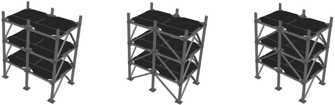
Figure 4. MTB2 building: a) SMF configuration (left), b) BRB-1 configuration (center), and c) BRB-2 configuration (right).
Summary
The Jupyter Notebooks developed for use through DesignSafe will facilitate the viewing and analysis of data sharing with collaborators from testing through data publication. A key advantage is the cloud-based approach that facilitates interactive data viewing and analysis in a report format without having to download large datasets. These tools are intended to make data more readily accessible and promote data reuse. The Jupyter Notebook presented here includes routines to evaluate the performance of the shake table and carry out system identification of structural models.
References
- Rathje et al. (2020) “Enhancing research in natural hazard engineering through the DesignSafe cyberinfrastructure”. Frontiers in Built Environment, 6:213.
- Vega et al (2020) “Implementation of real-time hybrid shake table testing using the UCSD large high-performance outdoor shake table”. Int. J. Lifecycle Performance Engineering, Vol. 4, p.80-102.
- Vega et al. (2018) "Five story building with tunned mass damper", in NHERI UCSD Hybrid Simulation Commissioning. DesignSafe-CI.
- Mosqueda et al. (2017) “Seismic Response of Base Isolated Buildings Considering Pounding to Moat Walls”. Technical report MCEER-13-0003.
- Van Den Einde et al (2020) “NHERI@ UC San Diego 6-DOF Large High-Performance Outdoor Shake Table Facility.” Frontiers in Built Environment, 6:181.
- Masroor et al. (2010) "Limit State Behavior of Base Isolated Structures: Fixed Base Moment Frame", DesignSafe-CI.
- Vega et al (2020), “Implementation of real-time hybrid shake table testing using the UCSD large high-performance outdoor shake table”. Int. J. Lifecycle Performance Engineering, Vol. 4, p.80-102.
- Brandenberg, S., J., & Yang, Y. (2021) "ucla_geotech_tools: A set of Python packages developed by the UCLA geotechnical group" (Version 1.0.2) [Computer software].
- Virtanen et al (2020) “SciPy 1.0: Fundamental Algorithms for Scientific Computing in Python”. Nature Methods, 17, 261–272.
- Chopra A. K., Dynamics of Structures. Harlow: Pearson Education, 2012.
- Morano M., Liu J., Hutchinson T. C., and Pantelides C.P. (2021), “Design and Analysis of a Modular Test Building for the 6-DOF Large High-Performace Outdoor Shake Table”, 17th World Conference on Earthquake Engineering, Japan.
- Mosqueda G, Guerrero N, Schmemmer Z., Lin L, Morano M., Liu J., Hutchinson T, Pantelides C P. Jupyter Notebooks for Data workflow of NHERI Experimental Facilities. Proceedings of the 12th National Conference in Earthquake Engineering, Earthquake Engineering Research Institute, Salt Lake City, UT. 2022.
Shake Table Data Analysis Using ML
Leveraging Machine Learning for Identification of Shake Table Data and Post Processing
Kayla Erler – University of California San Diego
Gilberto Mosqueda – University of California San Diego
Key Words: machine learning, shake table, friction, data modeling
Resources
Jupyter Notebooks
The following Jupyter notebooks are available to facilitate the analysis of each case. They are described in details in this section. You can access and run them directly on DesignSafe by clicking on the "Open in DesignSafe" button.
| Scope | Notebook |
|---|---|
| CASE 0 Preprocessing Visualization | Case 0 PreprocessingVisualization.ipynb |
| CASE 1 Linear Regression | Case 1 LinearRegression.ipynb |
| CASE 2 Deep Neural Network (DNN) Regression | Case 2 DNN.ipynb |
DesignSafe Resources
The following DesignSafe resources were used in developing this use case.
Additional Resources
- Jupyter Notebook and Python scripts on GitHub
- Caltrans Seismic Response Modification Device (SRMD) Test Facility
- Shortreed et al. (2001) "Characterization and testing of the Caltrans Seismic Response Modification Device Test System". Phil. Trans. R. Soc. A.359: 1829–1850
Description
This series of notebooks provides example applications of machine learning for earthquake engineering, specifically for use with experimental data derived from shake tables. Jupyter notebooks are implemented in a generalized format with modularized sections to allow for reusable code that can be readily transferable to other data sets. For complex nonlinear regression, a common method is to form a series of equations that accurately relates the data features to the target through approaches such as linear regression or empirical fitting. These notebooks explore the implementation and merits of several traditional approaches compared with higher level deep learning.
Linear regression, one of the most basic forms of machine learning, has many advantages in that it can provide a clear distinct verifiable solution. However, linear regression in some instances may fall short of achieving an accurate solution with real data. Additionally, this process requires many iterations to find the correct relationship. Therefore, it may be desirable to employ a more robust machine learning model to eliminate user time spent on model fitting as well as to achieve enhanced performance. The trade-off with using these algorithms is reduction in clarity of the derived relationships. To demonstrate an application of Machine Learning using Jupyter Notebooks in DesignSafe, models are implemented here for the measured forces in a shake table accounting for friction and inertial forces. Relatively robust data sets exist for training the models that make this a desirable application.
Implementation
Three notebooks are currently available for this project. The first, CASE 0, outlines the pre-processing that has been performed on the data before the model fitting procedures are conducted. CASE 1 contains details of the algorithms and theory for the linear regression model with several handy implementation tools to streamline model fitting for this or any other project. CASE 2 contains a deep neural network with an automated hyperparameter tuning algorithm. The notebooks are thoroughly commented with in depth details on their use and how they can be modified for use with other data sets on the DesignSafe platform. The user should review the notebooks for more instructive details. Note, for the deep neural network, if a wide range of hyperparameters is being used for tuning, and the dataset is large, tuning may take a significant amount of computational time when run on CPU. If a user gains access to the HPC available on the DesignSafe platform, the software is set up to be able to train on GPU when available.
Citations and Licensing
- Erler et al. (2024) "Leveraging Machine Learning Algorithms for Regression Analysis in Shake Table Data Processing". WCEE2024
- Rathje et al. (2017) "DesignSafe: New Cyberinfrastructure for Natural Hazards Engineering". ASCE: Natural Hazards Review / Volume 18 Issue 3 - August 2017
- This software is distributed under the GNU General Public License
OpenSees Model Calibration
From Constitutive Parameter Calibration to Site Response Analysis
Pedro Arduino - University of Washington
Sang-Ri Yi - SimCenter, UC Berkeley
Aakash Bangalore Satish - SimCenter, UC Berkeley
Key Words: quoFEM, OpenSees, Tapis, Python
A collection of educational notebooks to introduce model-parameter calibration and site response analysis using OpenSees in DesignSafe-CI.
Resources
Jupyter Notebooks
The following Jupyter notebooks are made available to facilitate the analysis of each case. They are described in detail in this section. You can access and run them directly on DesignSafe by clicking on the "Open in DesignSafe" button.
| Site Response | Notebook |
|---|---|
| FreeField Response | freeFieldJupyterPM4Sand_Community.ipynb |
| quoFEM | Notebook |
|---|---|
| Sensitivity analysis | quoFEM-Sensitivity.ipynb |
| Bayessian calibration | quoFEM-Bayesian.ipynb |
| Forward propagation | quoFEM-Propagation.ipynb |
DesignSafe Resources
The following DesignSafe resources were used in developing this use case.
- DesignSafe - Jupyter notebooks on DS Juypterhub
- SimCenter - quoFEM
- Simulation on DesignSafe - OpenSees
Background
Citation and Licensing
-
Please cite Aakash B. Satish et al. (2022) to acknowledge the use of resources from this use case.
-
Please cite Sang-Ri Yi et al. (2022) to acknowledge the use of resources from this use case.
-
Please cite Chen, L. et al. (2021) to acknowledge the use of resources from this use case.
-
Please cite Rathje et al. (2017) to acknowledge the use of DesignSafe resources.
-
This software is distributed under the GNU General Public License.
Description
Seismic site response refers to the way the ground responds to seismic waves during an earthquake. This response can vary based on the soil and rock properties of the site, as well as the characteristics of the earthquake itself.
Site response analysis for liquefiable soils is fundamental in the estimation of demands on civil infrastructure including buildings and lifelines. For this purpose, current state of the art in numerical methods in geotechnical engineering require the use of advance constitutive models and fully couple nonlinear finite element (FEM) tools. Advanced constitutive models require calibration of material parameters based on experimental tests. These parameters include uncertainties that in turn propagate to uncertenties in the estimation of demands. The products included in this use-case provide simple examples showing how to achieve site response analysis including parameter identification and uncertainty quantification using SimCenter tools and the DesignSafe cyber infrastructure.

Fig.1 - Site response problem
Implementation
This use-case introduces a suite of Jupyter Notebooks published in DesignSafe that navigate the process of constitutive model parameter calibration and site response analysis for a simple liquefaction case. They also introduce methods useful when using DesignSafe infrastructure in TACC. All notebooks leverage existing SimCenter backend functionality (e.g. Dakota, OpenSees, etc) implemented in quoFEM and run locally and in TACC through DesignSafe. The following two pages address these aspects, including:
-
Site response workflow notebook: This notebook introduces typical steps used a seismic site response analysis workflow taking advantage of Jupyter, OpenSees, and DesignSafe-CI.
-
quoFEM Notebooks: These notebooks provide an introduction to uncertainty quantification (UQ) methods using quoFEM to address sensitivity, Bayesian calibration, and forward propagation specifically in the context of seismic site response. Three different analysis are discussed including:
a. Global sensitivity analysis This notebook provides insight into which model parameters are critical for estimating triggering of liquefaction.
b. Parameter calibration notebook: This notebook is customized for the PM4Sand model and presents the estimation of its main parameters that best fit experimental data as well as their uncertainty.
c. Propagation of parameter undertainty in site response analysis notebook: This notebook introduces methods to propagate material parameter uncertainties in site reponse analysis.